Attention Is All You Need: The Paper That Revolutionized AI
In June 2017, eight researchers from Google Brain and Google Research published a paper that would fundamentally reshape artificial intelligence. Titled “Attention Is All You Need,” it introduced the Transformer architecture—a model that discarded the conventional wisdom of sequence processing and replaced it with something elegantly simple: pure attention.
The numbers tell the story. As of 2025, this single paper has been cited over 173,000 times, making it one of the most influential works in machine learning history. Today, nearly every large language model you interact with—ChatGPT, Google Gemini, Claude, Meta’s Llama—traces its lineage directly back to this architecture.
But here’s what makes this achievement remarkable: it wasn’t about adding more layers, more parameters, or more complexity. It was about removing what had been considered essential for decades.
The Problem: Sequential Processing
Why RNNs Were Dominant (And Problematic)
Before 2017, the dominant approach for sequence tasks used Recurrent Neural Networks (RNNs), particularly Long Short-Term Memory (LSTM) networks and Gated Recurrent Units (GRUs). The idea was intuitive: process sequences one element at a time, maintaining a hidden state that captures information from previous steps.
Think of it like reading a book word by word, keeping a mental summary as you go.
The Fundamental Bottleneck: RNNs have an inherent constraint—they must process sequentially. The output at step t depends on the hidden state h_t, which depends on the previous state h{t-1}, which depends on h{t-2}, and so on. This creates an unbreakable chain.
From the paper:
“Recurrent models typically factor computation along the symbol positions of the input and output sequences. Aligning the positions to steps in computation time, they generate a sequence of hidden states h_t, as a function of the previous hidden state h_{t-1} and the input for position t.”
What this meant in practice:
- Training Speed: On a typical machine translation task with 4.5 million sentence pairs (WMT 2014 English-German), even the best RNN models took 5-6 days to train on powerful hardware.
- Parallelization Nightmare: You cannot process word 10 before processing word 9, even if you have 1,000 GPUs. It’s like a single-lane highway—no matter how many resources you add, the throughput is limited by the sequential dependency.
- Memory Dilution: The longer your sequence, the harder it is for the model to remember important information from the beginning. This is called the “vanishing gradient problem.” Information from position 1 gets progressively diluted by the time you reach position 100.
- Long-Range Dependencies: If you want to understand how word 2 relates to word 95, the signal has to travel through 93 intermediate steps. Each step is an opportunity for information loss.
Attempted Solutions Before Transformers
Researchers had tried other approaches:
Convolutional Sequence-to-Sequence (ConvS2S): Used convolutional networks instead of RNNs. Problem: To connect distant positions, you need O(n/k) convolutional layers (where n is sequence length and k is kernel size). This means more layers and longer “path lengths” for information to travel. Extended Neural GPU & ByteNet: Other convolutional approaches with similar trade-offs.
The paper notes these approaches attempted to parallelize, but all had significant limitations. ConvS2S was faster than RNNs, but still limited. And none could match the quality of attention-augmented RNNs.
The Solution: Self-Attention
What is Attention?
Imagine you’re in a crowded coffee shop. Many conversations are happening, but you can focus your listening attention on one person. You’re not ignoring others, but you’re weighting your perception toward one source.
In neural networks, attention is a mechanism that learns which parts of the input are most important for the task at hand. It’s learned, dynamic, and task-specific.
The paper defines it simply:
“An attention function can be described as mapping a query and a set of key-value pairs to an output, where the query, keys, values, and output are all vectors. The output is computed as a weighted sum of the values, where the weight assigned to each value is computed by a compatibility function of the query with the corresponding key.”
 Source: Internet
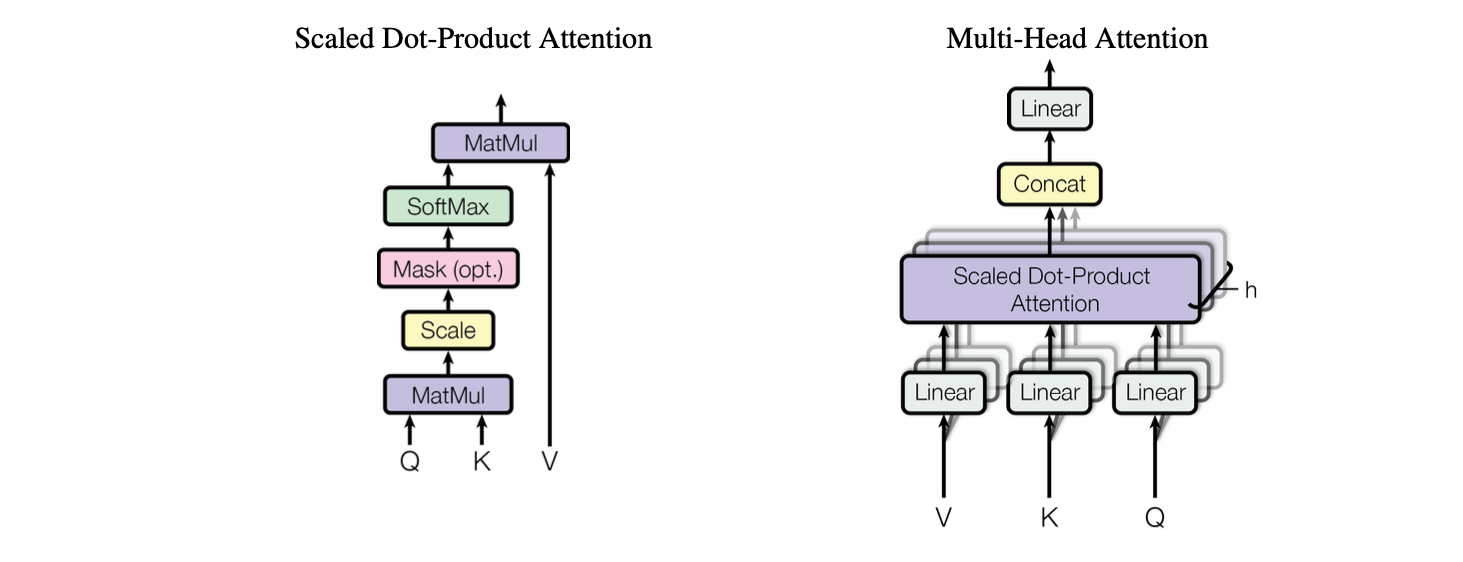
Scaled Dot-Product Attention: The Core Formula
The paper introduces “Scaled Dot-Product Attention,” which is the building block of everything:
Attention(Q, K, V) = softmax(QK^T / √d_k) VLet’s break this down step by step:
Step 1: Inputs
- Q (Query): “What am I looking for?” Shape: (batch, seq_len, d_k)
- K (Key): “What could I match?” Shape: (batch, seq_len, d_k)
- V (Value): “What information do I contain?” Shape: (batch, seq_len, d_v)
For self-attention, all three come from the same source (the output of the previous layer).
Step 2: Compute Compatibility Scores
QK^T produces a matrix showing how much each query relates to each key. If you have a sequence of 10 words, this creates a 10×10 matrix.
Step 3: Scaling The scores are divided by √d_k. Why? The paper explains:
“While for small values of d_k the two mechanisms perform similarly, additive attention outperforms dot product attention without scaling for larger values of d_k. We suspect that for large values of d_k, the dot products grow large in magnitude, pushing the softmax function into regions where it has extremely small gradients.”
In practice, they use d_k = 64, so the scaling factor is 1/√64 = 1/8.
Step 4: Softmax for Weights
softmax() converts the scores into weights that sum to 1. Each weight represents “how much attention to pay” to each position.
Step 5: Combine Values Multiply by V and sum. Positions with high attention weights contribute more to the output.
The Beauty: All n words can be processed in parallel. Position 10 doesn’t wait for position 9.
Why Multiple Heads Matter
Here’s where it gets powerful. The paper found that a single attention function isn’t enough. They introduced Multi-Head Attention:
MultiHead(Q, K, V) = Concat(head_1, ..., head_h) W^O

where head_i = Attention(QW^Q_i, KW^K_i, VW^V_i)
What does this mean? The model learns h different linear projections of Q, K, and V, performs attention on each separately, and concatenates the results.
From the paper:
“Multi-head attention allows the model to jointly attend to information from different representation subspaces at different positions. With a single attention head, averaging inhibits this.”
In the original Transformer:
- h = 8 parallel attention heads
- d_k = d_v = 512/8 = 64 for each head
- Total computation is similar to single-head attention, but you get 8 different learned representations
Practical interpretation: Different heads learn different patterns:
- Head 1 might focus on verb-object relationships
- Head 2 might focus on adjective-noun relationships
- Head 3 might track pronouns back to their referents
- And so on…
The attention visualizations in the paper (Figures 3-5) show this beautifully. Head 5 in layer 5 learns to capture the phrase “making…more difficult” by connecting distant words. Other heads perform anaphora resolution (connecting “its” to “Law”).
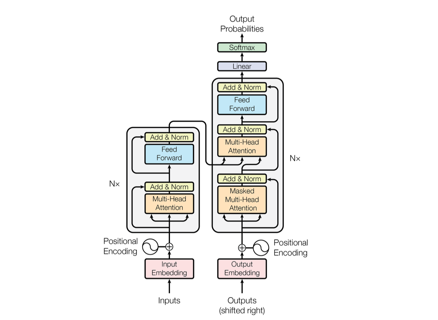
Transformer Architecture
Overview
The Transformer has a classic encoder-decoder structure:
- Encoder: Transforms input sequence into rich representations
- Decoder: Generates output sequence using encoder representations
 Source: Internet
But unlike previous encoder-decoder models, it uses only attention (and feed-forward networks) for both.
The Encoder: 6 Identical Layers
Each encoder layer contains:
- Multi-Head Self-Attention: All 8 heads process simultaneously
- Feed-Forward Network: Applied to each position separately
- Residual Connections & Layer Normalization around each sub-layer
The output of each sub-layer is:
LayerNorm(x + Sublayer(x))Key specifications:
- N = 6 stacked layers
- d_model = 512 (dimension of all outputs)
- h = 8 attention heads
- d_k = d_v = 64 per head
The Decoder: 6 Identical Layers with Masking
The decoder has the same 6 layers, plus one crucial difference:
- Masked Multi-Head Self-Attention on decoder positions
- Encoder-Decoder Attention: Queries from decoder, Keys/Values from encoder
- Feed-Forward Network
The Masking: The paper states:
“We also modify the self-attention sub-layer in the decoder stack to prevent positions from attending to subsequent positions. This masking, combined with fact that the output embeddings are offset by one position, ensures that the predictions for position i can depend only on the known outputs at positions less than i.”
In practice, this means setting future positions to -∞ in the softmax. This maintains the “auto-regressive” property—you generate one word at a time, without cheating by looking ahead.
Position-Wise Feed-Forward Networks
Between attention layers sits a feed-forward network:
FFN(x) = max(0, xW_1 + b_1)W_2 + b_2This is applied to each position separately and identically. Specifications:
- d_model = 512 (input/output dimension)
- d_ff = 2048 (inner layer dimension)
- ReLU activation in between
Interestingly, this is equivalent to two 1×1 convolutions.
Positional Encoding: Telling the Model About Order
Here’s a subtle but critical detail: attention mechanisms don’t inherently understand word order. “Dog bites man” and “man bites dog” would be processed the same without additional information.
The solution: Positional Encodings (sinusoidal):
PE_(pos, 2i) = sin(pos / 10000^(2i/d_model))
PE_(pos, 2i+1) = cos(pos / 10000^(2i/d_model))
Where:
- pos is the position in the sequence (0, 1, 2, …)
- i is the dimension index (0 to 255 for d_model=512)
Each dimension gets a sinusoid at different frequencies. The wavelengths form a geometric progression from 2π to 10,000·2π.
Why sine and cosine? The paper hypothesized this allows the model to easily learn relative position offsets since for any fixed offset k, PE{pos+k} can be represented as a linear function of PE{pos}.
The paper tested learned positional embeddings (Table 3, row E) and found nearly identical results, so the sinusoidal choice is more theoretical. But sinusoids have an advantage: they can extrapolate to longer sequences than seen during training.
The Three Applications of Attention
The paper explicitly lists three ways attention is used:
Encoder-Decoder Attention: Queries from decoder layer, Keys/Values from encoder output. Allows each decoder position to see all input positions.
Encoder Self-Attention: All of Q, K, V from the same encoder layer. Each position attends to all positions in the previous encoder layer.
Decoder Self-Attention: Self-attention with masking. Each position can only attend to previous positions (and itself).
Why Attention Works Better
The paper provides a systematic comparison in Table 1, examining three criteria:
1. Computational Complexity Per Layer
| Layer Type | Complexity |
|---|---|
| Self-Attention | O(n² · d) |
| Recurrent | O(n · d²) |
| Convolutional | O(k · n · d²) |
When sequence length n < representation dimension d (common with word-piece encoding), self-attention is faster than recurrent layers.
For WMT translation tasks using byte-pair encoding:
- n (sequence length) ≈ 50-200 tokens
- d (dimension) = 512
So n < d, making self-attention win.
2. Sequential Operations Required
| Layer Type | Sequential Operations |
|---|---|
| Self-Attention | O(1) |
| Recurrent | O(n) |
| Convolutional | O(1) for normal, O(logk(n)) for dilated |
This is the parallelization advantage. Self-attention can process all positions simultaneously. RNNs must process sequentially.
3. Path Length for Long-Range Dependencies
| Layer Type | Maximum Path Length |
|---|---|
| Self-Attention | O(1) |
| Recurrent | O(n) |
| Convolutional | O(logk(n)) or O(n/k) |
This is critical. To learn that position 1 relates to position 100:
- Self-Attention: Direct connection in one step
- RNN: Must travel through 99 intermediate steps
- CNN: Must stack multiple layers
Shorter paths → easier to learn long-range dependencies.
Results & Impact
Machine Translation Performance
The paper evaluated on two benchmarks: WMT 2014 English-German (EN-DE) and English-French (EN-FR).
English-to-German (EN-DE):
| Model | BLEU | Training Cost (FLOPs) | Training Time |
|---|---|---|---|
| GNMT + RL (prev. best) | 24.6 | 2.3 × 10¹⁹ | ~5 days |
| ConvS2S (ensemble) | 26.36 | 7.7 × 10¹⁹ | Higher |
| Transformer (base) | 27.3 | 3.3 × 10¹⁸ | 12 hours |
| Transformer (big) | 28.4 | 2.3 × 10¹⁹ | 3.5 days |
Improvement: +2.0 BLEU over previous best (including ensembles), at a fraction of training cost.
English-to-French (EN-FR):
| Model | BLEU | Training Time |
|---|---|---|
| Deep-Att + PosUnk Ensemble | 40.4 | High |
| GNMT + RL Ensemble | 41.16 | ~6 days |
| Transformer (big) | 41.8 | 3.5 days |
Improvement: Beats all previous models with less than ¼ training cost.
Key Numbers
- Hardware: 8 NVIDIA P100 GPUs
- Base model training time: 100,000 steps = 12 hours (0.4 seconds per step)
- Big model training time: 300,000 steps = 3.5 days (1.0 seconds per step)
- Dataset (EN-DE): 4.5 million sentence pairs
- Dataset (EN-FR): 36 million sentences
- Vocabulary (EN-DE): 37,000 tokens (byte-pair encoding)
- Vocabulary (EN-FR): 32,000 tokens (word-piece)
Generalization Beyond Translation
The paper also tested English constituency parsing (Penn Treebank):
| Model | WSJ Only | Semi-Supervised |
|---|---|---|
| Previous best (discriminative) | 91.7 | 92.1 |
| Transformer (4 layers) | 91.3 | 92.7 |
Despite no task-specific tuning, the Transformer achieved state-of-the-art on semi-supervised parsing and competitive results on WSJ-only. This proved the architecture was generalizable.
Technical Deep Dive
Model Variants & Ablation Study
The paper conducted extensive ablations (Table 3) to understand which components matter:
Multi-Head Variations (Rows A):
- 1 head: -0.9 BLEU
- 4 heads with h=128: No degradation
- 8 heads with h=64: Best (baseline)
- 16 heads with h=32: -0.4 BLEU
- 32 heads with h=16: -0.4 BLEU
Finding: Single-head attention hurts, but too many heads also degrades performance. Eight is optimal.
Attention Key Dimension (Rows B):
- d_k = 256/32 = 8: Worse
- d_k = 64 (baseline): Best
Finding: Smaller keys hurt model quality. The compatibility function needs sufficient dimensionality.
Model Size (Rows C, D):
- d_model = 256: Much worse
- d_model = 1024: Better but slower
- d_ff = 1024: Better
- d_ff = 4096: Even better (but more compute)
Finding: Larger models are better, as expected.
Regularization (Rows D):
- P_drop = 0.0: Severe overfitting
- P_drop = 0.1: Best for base model
- P_drop = 0.3: Better for larger models
Positional Encoding (Row E):
- Sinusoidal: 25.8 BLEU
- Learned embedding: 25.7 BLEU
Finding: Nearly identical, validating sinusoidal choice.
Training Details
Optimizer: Adam with β₁ = 0.9, β₂ = 0.98, ε = 10⁻⁹
Learning Rate Schedule:
lrate = d_model^(-0.5) · min(step_num^(-0.5), step_num · warmup_steps^(-1.5))With warmup_steps = 4000. This increases learning rate linearly for first 4000 steps, then decreases proportionally to step-0.5.
Regularization Techniques:
- Residual Dropout: Applied to all sub-layer outputs before adding residual connection. P_drop = 0.1 for base model.
- Label Smoothing: ε_ls = 0.1. This prevents model from becoming overconfident in predictions.
Inference: Beam search with beam size = 4, length penalty α = 0.6. Model parameters averaged over last 5-20 checkpoints.
Understanding the Impact
Why This Mattered
The Transformer’s success opened new possibilities:
- Massive Scale: Without sequential constraints, you could train enormous models. GPT-1 (2018) had 117 million parameters. GPT-3 (2020) had 175 billion. Each could train faster due to Transformer parallelization.
- Transfer Learning: BERT (2018) showed you could pre-train Transformers on massive unlabeled text, then fine-tune for specific tasks. This revolutionized NLP.
Generality: The same architecture worked for:
- Machine translation
- Text summarization
- Question answering
- Parsing
- (Later) Computer vision (Vision Transformers, 2020)
- (Later) Protein folding (AlphaFold, 2020)
- (Later) Speech, audio, multimodal tasks
Efficiency: Training became faster and cheaper, democratizing AI research.
Modern Descendants
Every major language model today uses Transformer variants:
- GPT series (OpenAI): Decoder-only Transformer
- BERT (Google): Encoder-only Transformer
- T5 (Google): Full encoder-decoder
- GPT-4, Gemini, Claude, Llama: All Transformer-based
Limitations & Future Directions
The paper acknowledges limitations:
- Quadratic Complexity: Self-attention is O(n² · d). Long documents become expensive. The paper suggests sparse attention for very long sequences.
- Effective Resolution: Attention averaging can lose fine-grained information in long sequences.
- Generation Speed: Decoding is still sequential (generates one word at a time).
Future work suggested:
- Restricted self-attention to handle images, audio, video
- Local attention mechanisms
- Making generation less sequential
(Later work addressed these: Sparse Transformers, Longformer, Flash Attention, etc.)
Conclusion
“Attention Is All You Need” presented a deceptively simple idea: replace recurrence and convolution with pure attention. But this simplicity masked profound consequences.
The paper proved that:
- Sequential processing isn’t necessary for sequence understanding
- Parallelization matters in practice for training speed
- Simpler architectures can outperform complex ones
- Elegant solutions often beat engineered complexity
The eight authors—Ashish Vaswani, Noam Shazeer, Niki Parmar, Jakob Uszkoreit, Llion Jones, Aidan Gomez, Łukasz Kaiser, and Illia Polosukhin—changed AI forever.
Nearly a decade later, we’re still discovering applications and improvements based on their core insight. Every conversation with ChatGPT, every Google search result, every code completion in your IDE—all trace back to this paper’s ideas.
The lesson transcends AI research: sometimes the breakthrough isn’t in complexity. It’s in finding the right abstraction that reveals hidden simplicity in what seemed complex before.
“Attention, after all, might be all we need.”